
August 12, 2020

Get accounting insights delivered directly to your inbox!
Many accountants have grown up using Excel, and continue to use it every day for calculations, graphing, pivots, and more. But even experienced Excel users can learn new tips and tricks to save hours each day.
In Part 1 of this series, we showed a useful trick for using text functions without editing. If you haven't read that post, we recommend starting there, because today's post continues where that one left off.
In Part 1, you used the LEFT, FIND, and MID functions to separate first and last names in a spreadsheet without using the Text-to-Columns functionality, which could break the link if the data is linked to a database, another spreadsheet, or a CSV file.
Now, our next step is to bring the full names back together again in the format we want: "FirstName LastName."
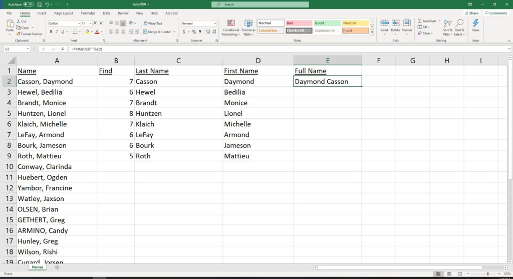
Start by naming the next empty column Full Name. A lot of people might use a CONCATENATE function here, but we'll show you a simpler way. In the first cell, type the following formula:
What this formula does is take whatever is in cell D2, puts a space after it, and then gives you whatever is in cell C2. Then you hit enter and get . . . an odd result.

Now you have the person's first name, then a whole bunch of spaces, followed by the last name. If you click on cell A2 and look at the formula bar, you see there are a whole bunch of unnecessary spaces. This happens a lot. Of course, you could go through your entire list and manually delete all those extra spaces every time they appear. But that would take a lot of time, and it's completely unnecessary.
Excel's TRIM function edits down all of those unnecessary spaces down to one space. To use it, we modify our simple formula in Step 1 to add the TRIM function, like this:
When you hit enter, you see it removes all those extra spaces.
Now that our functions are looking good, we can copy the formulas in each column all the way down.
(If you want a fast way to copy your formula across hundreds, thousands, or even millions of rows, check out our free webinar: Excel-lent Tips & Tricks.)
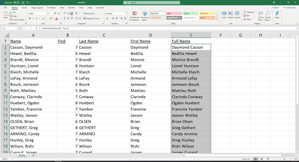
But then you notice some of the names on your list are in all caps. You might already be familiar with the UPPER function that turns everything in your text to uppercase, or the LOWER function that converts everything to lowercase. But since these are names, we want to use a function that capitalizes the first letter of the name, and puts the rest of the letters in lowercase. Fortunately, Excel has just the right function for that.
We don't need to create a separate column for this function. We can simply enclose the entire formula in column E within the PROPER function, like this:
When you copy the formula down your entire column, you'll see all those capital letters have been changed to proper names.
Now, you could be done with this spreadsheet; but if it bothers you to have all of these extra columns instead of one column with one formula, rest assured that it's possible to combine all four of these functions into one, and delete all of those extra columns.
For that, and some other helpful ways you can use the Data Fill function, you'll need to check out our free webinar: Excel-lent Tips & Tricks!
In the meantime, stay tuned for Part 3 of this series, where we'll show you how to calculate bonuses using VLOOKUP functions.


.svg)
